Physical organization¶

This page summarizes common on-disk organization and indexing techniques.

Throughout, let $B$ be the page (block) size in bytes and $H$ the page overhead. Let $V$ be the size of a search-key value, $P$ the size of a page pointer, and $R$ the size of a record identifier (record pointer).

ISAM¶

ISAM structure

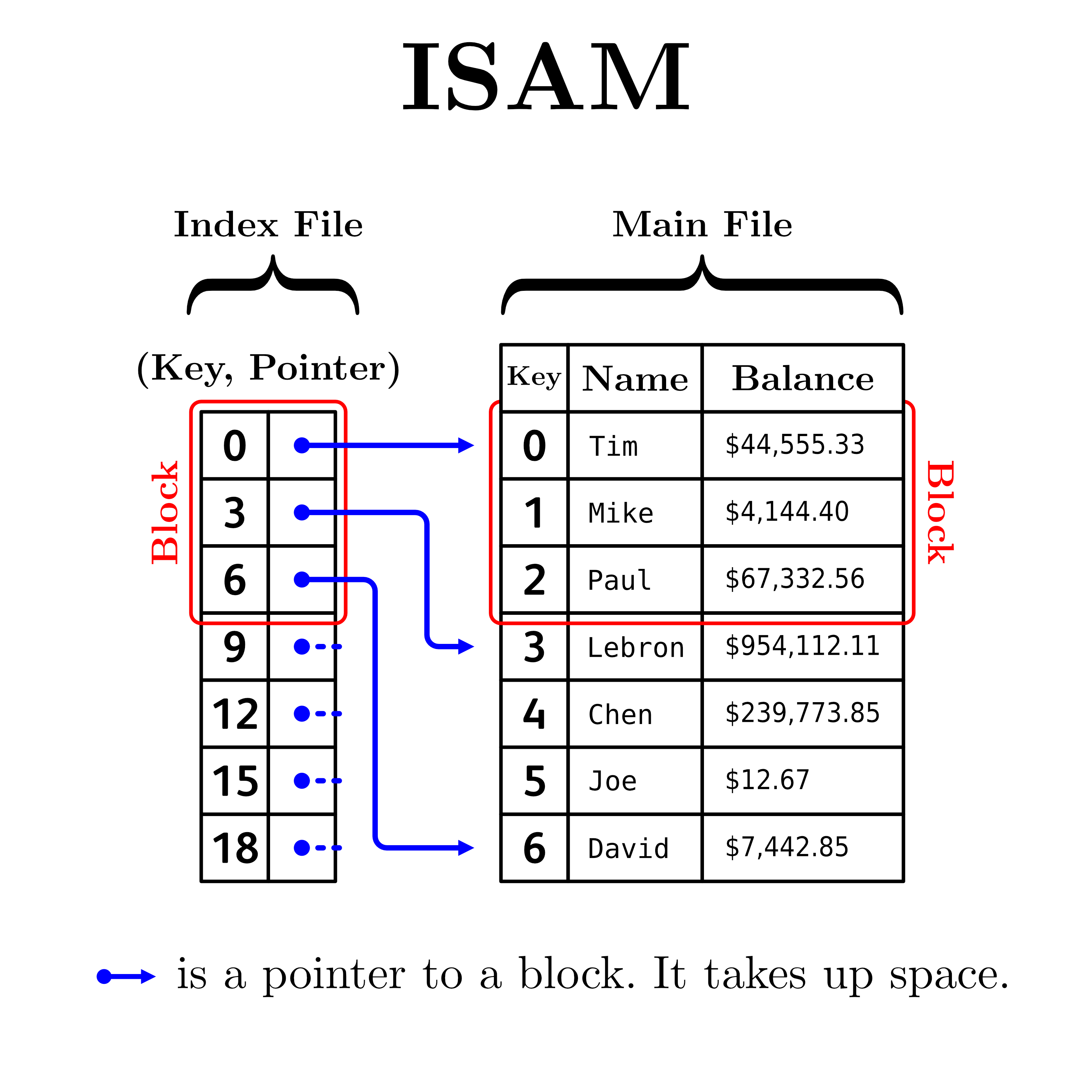
ISAM (Indexed Sequential Access Method) is a static file organization that combines the benefits of sequential storage (for range scans) and indexed access (for fast lookups). It was widely used in early database systems.

How it works¶

Basic concept:

Records are stored sorted by key in the primary file (data blocks)
A static index is built on top to provide direct access to blocks
The index stores (key, pointer) pairs: the smallest key in each block + a pointer to that block
The index itself can be multi-level (like a tree) for large files
When blocks fill up, overflow pages are chained to handle new insertions

Key characteristic - STATIC:

The index structure is built once and never reorganized
Tree shape is fixed even as data grows
Performance degrades over time as overflow chains grow
Periodic rebuilding required to restore performance

Physical structure¶

Primary file:

Data blocks containing records sorted by search key
Each block holds multiple records
Blocks are stored sequentially on disk

Index file:

Sparse index: one entry per data block (not per record)
Each index entry: (smallest key in block, pointer to block)
Can be multi-level: leaf index → intermediate levels → root

Overflow pages:

Chained from primary blocks when they become full
Not indexed - must be scanned sequentially
Cause performance degradation

Structure diagram:

Index Level 2 (Root):    [20 | 60]
                          /        \
Index Level 1:      [10|15|20]   [30|45|60]
                     / | \  \      / |  \  \
Primary Blocks:    B1 B2 B3 B4   B5 B6 B7 B8
                      |
Overflow:          [overflow] → [overflow]

Operations¶

Search for key $K$:

Start at root of index
Binary search within each index node to find child pointer
Follow pointers down to leaf index level
Follow pointer to data block
Scan data block (and overflow chain if needed)
Cost: $\lceil \log_2(N_{\text{blocks}}) \rceil + 1$ (index levels + data block)

Range scan (keys $K_1$ to $K_2$):

Use index to find starting block
Scan blocks sequentially (they're sorted!)
Cost: $\lceil \log_2(N_{\text{blocks}}) \rceil +$ (number of blocks in range)

Insert record with key $K$:

Find appropriate data block via index
If block has space: insert in sorted position
If block full: allocate overflow page, chain it, insert there
Index never changes (this is why it's static!)
Cost: search cost + 1-2 writes

Delete record:

Find and remove record
Index unchanged (even if block becomes empty)
Overflow pages can be reclaimed if they empty

Formulas¶

Given:

$N_{\text{rec}}$ = total number of records
$S_{\text{rec}}$ = size of each record in bytes
$K$ = size of the key in bytes
$B$ = block size in bytes
$P$ = pointer size in bytes

Records per block:

\[ \text{Records/Block} = \left\lfloor \frac{B}{S_{\text{rec}}} \right\rfloor \]

Number of primary file blocks:

\[ N_{\text{blocks}} = \left\lceil \frac{N_{\text{rec}}}{\text{Records/Block}} \right\rceil \]

Index entries per block:

Each index entry is (key, pointer) = $K + P$ bytes:

\[ \text{Entries/Index Block} = \left\lfloor \frac{B}{K + P} \right\rfloor \]

Number of index levels:

With fanout $f = \lfloor B/(K+P) \rfloor$, to index $N_{\text{blocks}}$ data blocks:

\[ \text{Levels} = \left\lceil \log_f(N_{\text{blocks}}) \right\rceil \]

For binary search in sorted index (when $f$ is large):

\[ \text{Levels} \approx \left\lceil \log_2(N_{\text{blocks}}) \right\rceil \]

File occupation:

Total space (ignoring overflows):

\[ \text{Occupation} = N_{\text{blocks}} \times B + \text{Index blocks} \times B \]

Binary search cost:

For an ISAM file with $N_{\text{blocks}}$ data blocks:

\[ \text{Cost}_{\text{binary}} = \left\lceil \log_2(N_{\text{blocks}}) \right\rceil + 1 \]

(Index traversal + final data block access)

Maximum records for given search cost:

Given maximum acceptable cost $C$ page accesses, maximum data blocks:

\[ N_{\text{blocks}}^{\max} = 2^{C-1} \]

Therefore maximum records:

\[ N_{\text{rec}}^{\max} = 2^{C-1} \times \left\lfloor \frac{B}{S_{\text{rec}}} \right\rfloor \]

Advantages and limitations¶

Advantages:

✓ Fast equality search via index
✓ Efficient range scans (data is sorted)
✓ Simple structure, easy to implement
✓ Good for read-heavy workloads with occasional inserts

Limitations:

✗ Static structure degrades with insertions (overflow chains)
✗ Periodic reorganization required (expensive!)
✗ Deletions don't reclaim index space
✗ Overflow chains hurt search performance
✗ Not suitable for write-heavy workloads

flowchart TB
  subgraph IDX[Index File]
    R[Root]
    I[Index level]
  end
  subgraph DATA[Primary File - Sorted data blocks]
    D1["Block 1<br/>keys: 10..19"]
    D2["Block 2<br/>keys: 20..29"]
    D3["Block 3<br/>keys: 30..39"]
  end
  subgraph OVF[Overflow pages]
    O1[Overflow for Block 2]
    O2[Overflow next]
  end

  R --> I
  I -->|< 20| D1
  I -->|20..29| D2
  I -->|>= 30| D3
  D2 -->|overflow| O1 --> O2

Hash-based organization¶

Hash-based organization

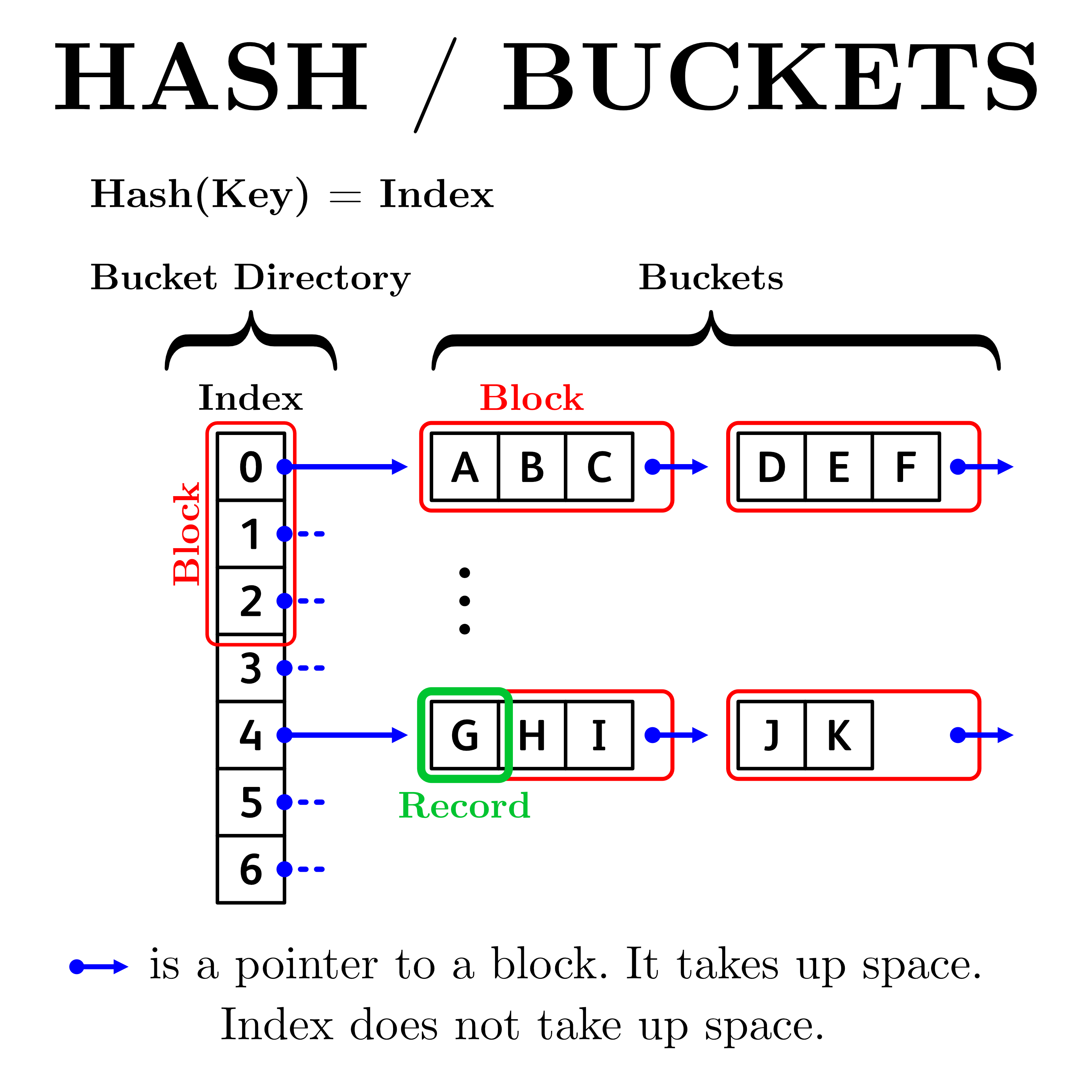
Hash-based organization uses a hash function to map search keys directly to physical storage locations. This provides extremely fast equality lookups but sacrifices the ability to perform efficient range queries.

How it works¶

Basic concept:

A hash function $h(K)$ maps each search key $K$ to a bucket number
Each bucket is a storage area (one or more disk pages) that holds records with keys that hash to that bucket
The hash function distributes records across $N_{\text{buckets}}$ buckets
To search for a record with key $K$: compute $b = h(K)$ and read bucket $b$

Example: With $h(K) = K \bmod 10$ and buckets 0-9:

Key 23 → bucket 3
Key 57 → bucket 7
Key 103 → bucket 3 (same as 23, a collision)

Physical structure¶

Each bucket consists of:

Primary page: The main page for that bucket
Overflow pages (optional): Linked pages when primary page fills up

A bucket page typically stores:

Header: Metadata (free space pointer, overflow pointer, etc.)
Data entries: Either:
- (key, record) pairs if the file is hash-organized
- (key, rid) pairs if this is a hash index on another file

Page layout:

┌─────────────────────────────────────┐
│ Header (H bytes)                    │
├─────────────────────────────────────┤
│ Entry 1: (key₁, data₁)              │
│ Entry 2: (key₂, data₂)              │
│ ...                                 │
│ Entry c: (keyc, datac)              │
├─────────────────────────────────────┤
│ Free space                          │
├─────────────────────────────────────┤
│ Pointer to overflow page (if any)   │
└─────────────────────────────────────┘

Operations¶

Search for key $K$:

Compute bucket number: $b = h(K)$
Read primary page of bucket $b$
Scan entries in page looking for $K$
If not found and overflow exists, follow overflow chain
Cost: 1 + (number of overflow pages to scan)

Insert record with key $K$:

Compute bucket number: $b = h(K)$
Read primary page of bucket $b$
If space available, insert entry into page
If page full, allocate overflow page and link it
Cost: 1 read + 1 write (+ overflow allocation if needed)

Delete record with key $K$:

Search for the record (as above)
Remove entry from page
If overflow pages become empty, deallocate them
Cost: similar to search + 1 write

Formulas¶

Given:

$N_{\text{rec}}$ = total number of records
$K$ = size of the key in bytes
$R$ = size of data/record pointer in bytes
$B$ = block (page) size in bytes
$H$ = page header/overhead in bytes
$N_{\text{buckets}}$ = number of hash buckets

Entries per bucket page:

Each entry is a (key, data) pair of size $K + R$ bytes:

\[ c = \left\lfloor \frac{B - H}{K + R} \right\rfloor \]

Average entries per bucket:

With uniform hash distribution:

\[ \bar{n} = \frac{N_{\text{rec}}}{N_{\text{buckets}}} \]

Load factor:

The load factor $\alpha$ indicates how full the hash table is:

\[ \alpha = \frac{N_{\text{rec}}}{N_{\text{buckets}} \times c} \]

$\alpha < 1$: Some buckets have free space
$\alpha = 1$: All primary pages full on average
$\alpha > 1$: Overflow pages are needed

Pages per bucket:

If a bucket contains $n_b$ entries:

\[ \text{Pages} = \left\lceil \frac{n_b}{c} \right\rceil \]

This includes the primary page plus any overflow pages.

Search cost:

Best case: 1 page access (key found in primary page)
Average case: $1 + \frac{\alpha - 1}{2}$ page accesses (if $\alpha > 1$)
Worst case: $1 +$ (length of overflow chain)

Static vs Dynamic Hashing¶

Static hashing:

Fixed $N_{\text{buckets}}$ decided at creation time
Hash function: $h(K) = K \bmod N_{\text{buckets}}$
Problem: As data grows, $\alpha$ increases → long overflow chains → poor performance
Solution: Periodically reorganize entire file with larger $N_{\text{buckets}}$

Dynamic hashing (extendible/linear):

$N_{\text{buckets}}$ grows/shrinks dynamically
Maintains $\alpha$ close to optimal (typically 0.7-0.8)
No full reorganization needed
More complex but scales better

Advantages and limitations¶

Advantages:

✓ Very fast equality search: $O(1)$ average time
✓ Fast insertion/deletion: $O(1)$ average time
✓ No index overhead (for hash-organized files)

Limitations:

✗ Cannot support range queries efficiently (must scan all buckets)
✗ Cannot support ordered access or sorting
✗ Performance degrades with high load factor (overflow chains)
✗ Hash function quality affects distribution

flowchart LR
  K["Key K"] --> H["h(K)"] -->|bucket_id| B["bucket b"]
  subgraph BUCKETS[Buckets]
    B0[Bucket 0]
    B1[Bucket 1]
    B2[Bucket 2]
    B3[Bucket 3]
  end
  B --> B2
  B2 -->|overflow| O1[Overflow] --> O2[Overflow]

B-tree¶

B-tree structure

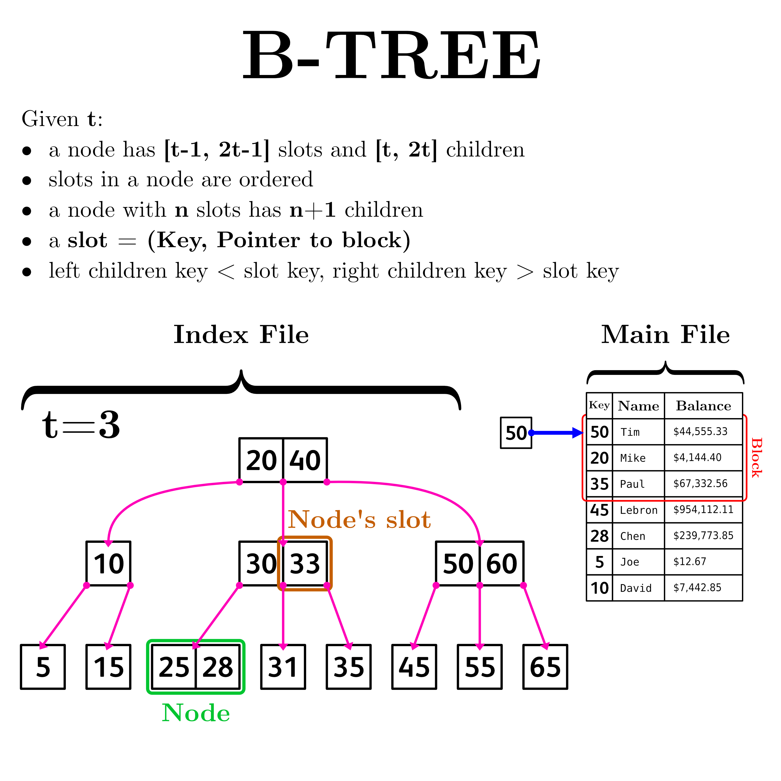
A B-tree is a self-balancing multiway search tree optimized for disk storage. Unlike ISAM, it dynamically reorganizes itself to maintain balance and good performance as data changes.

How it works¶

Basic concept:

Tree is always perfectly balanced: all leaves at same depth
Each node is stored in one disk page
Nodes contain multiple keys (not just one like binary trees)
Keys in a node are sorted
Each key has data associated with it (or pointer to data)
Internal nodes have child pointers separating key ranges

Key characteristic - DYNAMIC:

When a node fills up → split it into two nodes
When a node becomes too empty → merge it with sibling
Tree automatically rebalances during insertions/deletions
Height stays logarithmic: $O(\log_p N)$ where $p$ is fanout

Physical structure¶

Node layout:

Each node (stored in one page) contains: - Header: metadata, number of keys, etc. - $n$ keys: $k_1, k_2, ..., k_n$ (sorted) - $n+1$ child pointers: $p_0, p_1, ..., p_n$ - Data associated with each key (or record pointers)

Structure example:

Node structure with 3 keys:
┌────────────────────────────────────────────────┐
│ [p₀][k₁,data₁][p₁][k₂,data₂][p₂][k₃,data₃][p₃] │
└────────────────────────────────────────────────┘

Pointer meaning:
  p₀ → children with keys < k₁
  p₁ → children with keys between k₁ and k₂  
  p₂ → children with keys between k₂ and k₃
  p₃ → children with keys > k₃

Tree properties:

All leaves at the same depth $h$
Each node (except root) has between $\lceil p_{\max}/2 \rceil$ and $p_{\max}$ children
Root has at least 2 children (unless tree has only one node)
Keys stored in both internal nodes and leaves
Each internal node acts as a "router" to guide searches

Operations¶

Search for key $K$:

Start at root
Within node, find where $K$ falls among sorted keys:
If $K = k_i$ → found! Return data
If $k_i < K < k_{i+1}$ → follow pointer $p_i$ to child
Repeat until key found or reach leaf
Cost: $O(h)$ page reads = $O(\log_p N)$

Insert key $K$ with data:

Search to find appropriate leaf
Insert $(K, data)$ in sorted position in leaf
If leaf has space → done
If leaf is full (has $p_{\max}$ entries):
Split leaf into two nodes
Promote middle key to parent
If parent full → split parent recursively
May propagate up to root (increasing tree height)
Cost: $O(h)$ reads + $O(h)$ writes

Delete key $K$:

Search to find $K$
Remove $K$ from node
If node still has $\geq \lceil p_{\max}/2 \rceil$ entries → done
If node too empty:
Try to redistribute with sibling (borrow a key)
If sibling also minimal → merge with sibling
May propagate up (decreasing tree height)
Cost: $O(h)$ reads + $O(h)$ writes

Range scan ($K_1$ to $K_2$):

Search for $K_1$ to find starting point
Must traverse tree structure to find each key in range
Less efficient than B+ tree (no leaf linking)
Cost: $O(h \cdot k)$ where $k$ is number of results

Formulas¶

Given:

$V$ = size of a key value in bytes
$P$ = size of a pointer in bytes
$B$ = block size in bytes
$H$ = page header/overhead in bytes
$N_{\text{keys}}$ = total number of keys in the tree

Node space constraint:

A node with $p$ child pointers has $p-1$ keys. Total space:

\[ p \cdot P + (p-1) \cdot V \le B - H \]

Maximum fanout (order):

Solving for $p$:

\[ p_{\max} = \left\lfloor \frac{B - H + V}{P + V} \right\rfloor \]

Minimum fanout:

For all nodes except root (to guarantee balance):

\[ p_{\min} = \left\lceil \frac{p_{\max}}{2} \right\rceil \]

The root can have as few as 2 children.

Tree height:

Minimum height (all nodes full with $p_{\max}$ children):

\[ h_{\min} = \left\lceil \log_{p_{\max}}(N_{\text{keys}}+1) \right\rceil \]

Maximum height (all nodes minimal with $\lceil p_{\max}/2 \rceil$ children):

\[ h_{\max} = \left\lceil \log_{\lceil p_{\max}/2 \rceil}\left(\frac{N_{\text{keys}}+1}{2}\right) \right\rceil \]

Typically $h = 2$ to $4$ for millions of keys.

Search cost:

Equality search: $O(h)$ page reads
Typical: $h \approx \log_{p_{\max}} N$
Example: With $p_{\max} = 200$ and $N = 1,000,000$ keys: $$h \approx \log_{200}(10^6) \approx 2.6 \approx 3 \text{ levels}$$

Advantages and limitations¶

Advantages:

✓ Always balanced: guaranteed $O(\log N)$ performance
✓ Handles insertions/deletions efficiently
✓ No overflow pages or reorganization needed
✓ Good for dynamic datasets (frequent updates)
✓ High fanout → short trees → few disk accesses

Limitations:

✗ More complex than ISAM (split/merge logic)
✗ Range scans less efficient (no leaf linking)
✗ Keys stored in internal nodes waste space
✗ Internal nodes mix routing + data (less efficient)

flowchart TB
  R["20, 40"]
  C1["5, 12"]
  C2["25, 30"]
  C3["45, 50, 60"]

  R -->|< 20| C1
  R -->|20..39| C2
  R -->|>= 40| C3

B+ tree¶

B+ tree structure

TODO: B+ tree image

A B+ tree is a variant of the B-tree optimized for disk-based storage with these key differences:

All data entries in leaves: Internal nodes store only separator keys + pointers
Leaves are linked: Sequential linked list enables efficient range scans
Higher fanout: Internal nodes can store more pointers (no data overhead)
Duplicated keys: Keys may appear in both internal nodes and leaves

Organization¶

Given:

$V$ = size of a key value in bytes
$P$ = size of a pointer in bytes
$R$ = size of a record identifier in bytes
$B$ = block size in bytes
$H$ = page header/overhead in bytes
$N_{\text{rec}}$ = total number of records

Internal node fanout:

Internal nodes contain only keys and pointers, so:

\[ p_{\max} = \left\lfloor \frac{B - H + V}{P + V} \right\rfloor \]

Leaf node capacity:

Leaves store data entries $(K, \text{rid})$ of size $V+R$ plus one pointer to the next leaf:

\[ L = \left\lfloor \frac{B - H - P}{V + R} \right\rfloor \]

where the $-P$ accounts for the next-leaf pointer.

Alternatively, if the next-leaf pointer is not counted in the capacity:

\[ L = \left\lfloor \frac{B - H}{V + R} \right\rfloor \]

Number of leaf pages:

\[ N_{\text{leaves}} = \left\lceil \frac{N_{\text{rec}}}{L} \right\rceil \]

Tree height:

With $N_{\text{leaves}}$ leaf pages:

\[ h = \left\lceil \log_{p_{\max}}(N_{\text{leaves}}) \right\rceil \]

For $N_{\text{rec}}$ records:

\[ h = \left\lceil \log_{p_{\max}}\left(\left\lceil \frac{N_{\text{rec}}}{L} \right\rceil\right) \right\rceil \]

Search costs:

Equality search: $h+1$ page accesses (root to leaf)
Range query for $k$ results: $h + \lceil k/L \rceil$ page accesses
Pay root-to-leaf traversal once ($h$ pages)
Follow linked leaves ($\lceil k/L \rceil$ leaf pages)
Sequential scan: Very efficient due to linked leaves

Space utilization:

With typical fill factor of 67% (minimum occupancy):

\[ \text{Total pages} \approx \frac{N_{\text{rec}}}{0.67 \times L} + \text{internal nodes} \]

flowchart TB
  R["20, 40"]
  I1["10, 15"]
  I2["25, 30"]
  I3["45, 55"]

  L1[(Leaf: 1,5,9)]
  L2[(Leaf: 10,12,14)]
  L3[(Leaf: 15,18,19)]
  L4[(Leaf: 20,22,24)]
  L5[(Leaf: 25,27,29)]
  L6[(Leaf: 30,35,39)]
  L7[(Leaf: 40,44)]
  L8[(Leaf: 45,50,54)]
  L9[(Leaf: 55,60)]

  R --> I1
  R --> I2
  R --> I3

  I1 --> L1
  I1 --> L2
  I1 --> L3
  I2 --> L4
  I2 --> L5
  I2 --> L6
  I3 --> L7
  I3 --> L8
  I3 --> L9

  L1 <--> L2 <--> L3 <--> L4 <--> L5 <--> L6 <--> L7 <--> L8 <--> L9

A small sizing example¶

Let $B = 4096$, $H = 128$, and $V=P=R=8$ bytes.

For an internal node,

\[ p_{\max} = \left\lfloor \frac{B - H + V}{P + V} \right\rfloor = \left\lfloor \frac{4096 - 128 + 8}{8 + 8} \right\rfloor = \left\lfloor \frac{3976}{16} \right\rfloor = 248. \]

For a B+ tree leaf,

\[ L = \left\lfloor \frac{B - H - P}{V + R} \right\rfloor = \left\lfloor \frac{4096 - 128 - 8}{8 + 8} \right\rfloor = \left\lfloor \frac{3960}{16} \right\rfloor = 247. \]